A Simple Framework for Contrastive Learning of Visual Representations
A popular and useful framework for contrastive self-supervised learning known as SimCLR was introduced by Chen et. al.. The framework simplifies previous contrastive methods to self-supervised learning, and at the time was state-of-the-art at unsupervised image representation learning. The main simplification lies in the fact that SimCLR requires no specialised modules or additions to the architecture such as memory banks.
Architecture
As with previous contrastive methods, the architecture is a Siamese-like, as can be seen below:
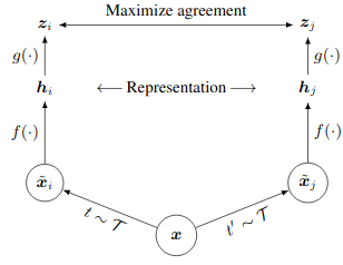
An input image \(x\) is sampled from the training dataset. Two random augmentations are then applied to this input image to produce two distinct views \(x_i\) and \(x_j\) of the same image. These two images are fed through the same encoder \(f\) to produce latent vectors \(h_i\) and \(h_j\). It should be noted that \(f\) is parameterised as a large CNN such as ResNet. Finallly, these latent vectors are fed through an MLP \(g\) (known as the projection head) to produce final latent vectors \(z_i\) and \(z_j\).
Although \(f\) may initially seem unnecessary, it has been shown empirically to improve performance versus just using \(h_i\) and \(h_j\) as the latent representations. Importantly, the supervision signal is computed using the projection head latent vectors \(z_i\) and \(z_j\), and not using the encoder latent vectors. Further, the encoder latent vectors are the ones used for downstream tasks (linear evaluation, etc.) after this self-supervised training.
Loss Function
Since this is a contrastive, the loss function is defined in such a way that it contrasts negative pairs of examples from positive pairs of examples (i.e. \(x_i\) and \(x_j\) are a positive pair of examples). This loss function is known as normalised temperature-scaled cross entropy (NT-Xent), and is defined as:
\[l_{i,j} = -\text{log} \frac{\text{exp}(\text{sim}(z_i, z_j) / \tau)}{\sum_{k=1}^{2N} 1\{k \neq i\} \text{exp}(\text{sim}(z_i, z_k) / \tau)}\]where \(\tau\) is the temperature, \(N\) is the minibatch size, and \(\text{sim}\) is the cosine similarity. With this loss, all pairs of examples in a minibatch are treated as negative examples, except for the single pair \(z_i, z_j\). This loss function works well in practise, but typically requires very large batch sizes to be effective.
Note that this is architecture and loss function are fully unsupervised.
Data Augmentations
The augmentations applied during training are 1. random cropping and resizing, 2. random colour distortions (in the form of brightness, hue, saturation, and contrast jitter), and 3. random Gaussian blurring. It should be noted that, for SimCLR, random cropping and colour jittering are crucial for good performance.
Consideration
Although SimCLR works well, there are a few drawbacks. Firstly, the computation needed to train the architecture to an acceptable level can be prohibitive. The batch size using in the paper is 4096 which means 8192 images are in each the batch for each training iterations.