All About Convex Hulls
The convex hull is a very important concept in geometry, and has many applications in fields such as computer vision, mathematics, statistics, and economics. Essentially, a convex hull of a shape or set of points is the smallest convex set that contains that shape or set of points. Many algorithms exist to compute a convex hull. Many of these algorithms have focused on the 2D or 3D case, however, the general \(d\)-dimensional case is of big interest in many applications.
It is important to first build up some background knowledge so that we can effectively talk about convex hulls. We will be working with the general \(d\)-dimensional case, but will visualise in 2D. First, we have the concept of a \(d\)-simplex, which is just a generalisation of the concept of a triangle to arbitrary dimensions (similar to what a cube is to a square or a hyperplane to a line). Additionally, a \(d\)-dimensional convex hull is represented by its vertices and “faces” (which are essentially \(d - 1\)-dimensional affine hyperplanes).
Consider a set of \(n\) points \(\mathcal{S} = \{\mathbf{x}_i \in \mathbb{R}^d\}_{i=1}^n\) for which we want to compute a convex hull.
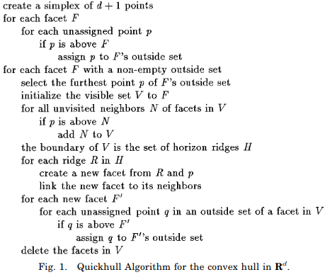
A very naive approach (that I strongly recommend against using) is the following. We simply consider all possible faces / hyperplanes that can be made using points from \(\mathcal{S}\), and choose only those faces where all other points lie only to one side of the face. In the below figure, F1 is one such face, since all other points lie to one side of the face. However, F2 is not, since points lie on both side of it. Thus F1 will be part of the convex hull, whereas F2 will not.
This naive algorithm is highly inefficient since all possible faces will need to be checked. This involves checking \(n \choose d\) possible faces. In order words, the computational complexity of this algorithm is \(\Theta({n \choose d})\).
A much more efficient algorithm for computing a convex hull is the quickhull algorithm. It is a popular algorithm for the general dimension case, and is indeed the implementation in the scipy package (which leverages the qhull library).
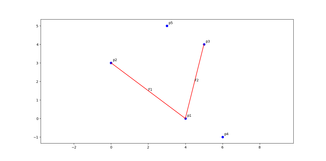
A key operation used in the quickhull algorithm is signed distance from a point to a hyperplane. We need it to be signed, since we want to know which side of the hyperplane /face the point lies. Formally, we can compute this signed distance for a point \(\mathbf{x}\) using the following:
\[\frac{\langle \mathbf{x}, \mathbf{n} \rangle - \langle \mathbf{p}, \mathbf{n} \rangle}{||\mathbf{n}||_2}\]where \(\mathbf{p}\) is a point that lies on the hyperplane, and \(\mathbf{n}\) is the hyperplane’s normal vector. This distance is visualised in the below figure.
The full algorithm is given below: