Human Action Recognition
In this post we will discuss the problem of human action recognition - an application of video analysis / recognition. The task is simply to identify a single action from a video. The typically setting is a dataset consisting of \(N\) action classes, where each class has a set of videos associated with it relating to that action. We will focus on the approaches typically taken in early action recognition research, and then focus on the current state-of-the-art approaches. There is a recurring theme in action recognition of extending conventional two-dimensional algorithms into three dimensions to accommodate for the extra (temporal) dimension when dealing with videos instead of images.
Early research tends to focus on hand-crafting features. The benefit of this is that you are incorporating domain knowledge into the features, which should increase performance. The high-level idea behind these approaches is as follows:
- Use interest point detection mechanism to localise points of interest to be used as the basis for feature extraction.
- Compute descriptions of these interest points in the form of (typically, gradient-based) descriptors.
- Quantise local descriptors into global video feature representations.
- Train an SVM of some form to learn to map from gloval video representation to action class.
Interest points are usually detected using a three-dimensional extension of the well-known Harris operator - space-time interest points (STIPs). However, in later research simple dense sampling was instead preferred for its resulting performance and speed. Interest points are also detected at multiple spatial and temporal scales to account for actions of differing speed and temporal extent. Descriptors are commonly computed within a local three-dimensional volume of the interest points (i.e. a cuboid). These descriptors are typically one of the following three (into some or other form): 1. histogram of oriented gradients; 2. histogram of optical flow; 3. motion boundary histograms.
The quantisation step to encode these local features into a global, fixed-length feature representation is usually done using either: 1. K-Means clustering using a bag-of-visual-words approach; or 2. Fisher vectors. Fisher vectors typically result in higher performance, but at a cost of dimensionality exploding. The normalisation applied to these features is important. The common approach was applying \(L_2\) normalisation, however power normalisation is preferred more recently. An SVM then learns the mapping to action classes from the normalised versions of the representations. The most successful of these hand-crafted approaches is iDT (improved dense trajectories). iDTs are often used in tandem with deep networks in state-of-the-art approaches as they are able to encode some pertinent, salient information about the videos / actions that is difficult for the networks to capture.
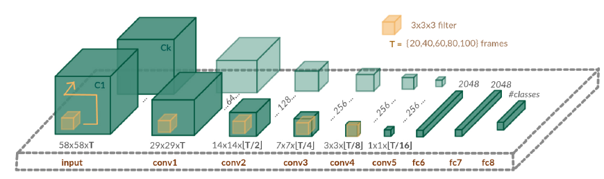
More recent research into action recognition has, unsurprisingly, been focused on deep learning. The most natural way to apply deep neural networks to video is to extend the successful 2D CNN architectures into the temporal domain by simply using 3D kernels in the convolutional layers and 3D pooling. This use of 3D CNNs is very common in this domain, although some research did attempt to process individual RGB frames with 2D CNN architectures. An example of a 3D CNN can be seen below.
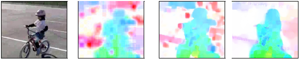
The most significant contribution to human action recognition using deep learning, however, was the introduction of additional cues to model the action. More concretely, the raw RGB videos are fed into one 3D CNN which will learn salient appearance features. Further, there is another network - a flow network - which learns salient motion features from optical flow videos. An optical flow video is computed by performing frame-by-frame dense optical flow on the raw video, and using the resulting horizontal and vertical optical flow vector fields as the “images” / “frames” of the flow video. This modeling process is based on the intuition that actions can naturally be decomposed into a spatial and temporal components (which will be modelled by the RGB and flow networks separately). An example of a optical flow field “frame” using different optical flow algorithms can be seen below (RGB frame, MPEG flow, Farneback flow, and Brox flow). The more accurate flow algorithms such as Brox and TVL-1, result in higher performance. However, they are much more intensive to compute, especially without their GPU implementations.
This two-network approach is the basis for the state-of-the-art approaches in action recognition such as I3D and temporal segment networks. Some research attempts to add additional cues to appearance and motion to model actions, such as pose.
It is important to note that when using deep learning to solve action recognition, massive computational resources are needed to train the 3D CNNs. Some of the state-of-the-art approaches utilise upwards of 64 powerful GPUs to train the networks. This is needed in particular to pre-train the networks on massive datasets like Kinetics to make use of transfer learning.
Another consideration to consider (using deep learning approaches particularly) is the temporal resolution of the samples used during training. The durations of actions vary hugely, and in order to make the system robust, the model needs to accommodate for this. Some approaches employ careful sampling of various snippets along the temporal evolution of the video so that the samples cover the action fully. Others employ a large temporal resolution for the sample - 60-100 frames. However, this increases computational cost significantly.
Some good resources and references can be found here: