Dimensionality Reduction
In machine learning, we often work with very high-dimensional data. For example, we might be working in a genome prediction context, in which case our feature vectors would contains thousands of dimensions, or perhaps we’re dealing in another context where the dimensions reach of hundreds of thousands or possibly millions. In such a context, one common way to get a handle on the data - to understand it better - is to visualise the data by reducing its dimensions. The can be done using conventional dimensionality reduction techniques such as PCA and LDA, or using manifold learning techniques such as t-SNE and LLE.
For the purposes of this post, let’s assume the input features are \(M\)-dimensional.
The most popular, and perhaps simplest, dimensionality reduction technique is principal components analysis (PCA). In it, we assume that the relationships between the variables / features are linear. “Importance” in the PCA algorithm is defined by variance. This assumption that variance is the important factor often holds (but not always!). To get the so-called principal components of the data, we find the orthogonal directions of maximum variance. These are the components that maximize the variance of the data.
We obtain these principal components via finding the eigen decomposition of the covariance matrix of the input matrix - that is, its eigenvalues and eigenvectors. Since computing the covariance matrix is often prohibitive to compute for a large number of features, the eigenvalues and eigenvectors are often found by using the SVD algorithm which decomposes the input matrix down into three separate matrices, two of which are the eigenvalues and eigenvectors. In this way, we need to directly compute the covariance matrix. The data must be centered in order for this SVD trick to work.
The \(N\) principal components are then the \(N\) eigenvectors with largest associated absolute eigenvalues. These are linear combinations of the input features, where is each feature contributes different amounts to the principal component. If there are strong linear relationships between the input variables, relatively few principal components will capture the majority of the variance in the data. However, if not much of the variance is captured by relatively few components, this does not necessarily mean that there are no relationships or underlying structure in the data - the structure might be in the form of non-linear interactiions and relationships. This is the reason non-linear dimensionality reduction (such as KPCA) and manifold learning techniques exist.
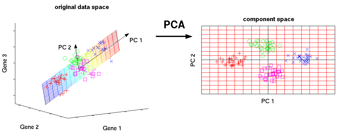
In the above image we can see that in the original, 3-dimensional, raw feature space, the clusters of data are separated quite nicely. The 4 groups are roughly linear separable. In the left plot, we can also see the first two pincipal components of the data - the two (orthogonal) directions / axes in which the data varies maximally with respect to variance. In the right plot, we can see the projection of the data into the 2-dimensional principal subspace. The data separates quite nicely into 4 distinct clusters. This suggests that the data has strong linear relationships.
Manifold learning allows us to estimate the hypothesised low-dimensional non-linear manifold (or set of manifolds) on which our high-dimensional data lies. Different manifold learning algorithms optimise for different criteria depending on what type of structure of the data they want to capture - local or global or a combination.
I’ll discuss one manifold learning technique. This technique - t-SNE - is popular in the machine learning research communited. t-SNE stands for t-distributed stochastic neighbour embedding. t-SNE spawns from a technique known as SNE (unsuprisingly known as stochastic neighbour embedding). SNE converts distances between data points in the original, high-dimensional space (termed datapoints) into conditional probabilities that represent similarities. These similarities are simply the probability that a datapoint \(x_i\) would pick a datapoint \(x_j\) as its neighbour if neighbours were picked in proportion to their probability density under a Gaussian centered at \(x_i\), which we denote as \(p_{ij}\). This means that for nearby points, this similarity is relatively high, and for widely-separated points this similarity approaches zero. The low-dimensional counterparts of the datapoints (known as the map points) are \(y_i\) and \(y_j\). We compute similar conditional probabilities (i.e. similarities) for these map points, which we denote \(q_{ij}\).
If these map points correctly model the similarities of the datapoints, we should have that \(p_{ij}\) is equal to \(q_{ij}\). Thus, SNE attempts to find the low-dimensional representation that minimizes the KL-divergence between these two conditional distributions. The problem with this approach is that the cost function is difficult to optimize, and it also suffers from the infamous crowding problem - the area of the low-dimensional map that is available to accomodate moderately-distant datapoints will not be nearly large enough compared with the area available to accomodate nearby datapoints. Thus, t-SNE is born.
t-SNE addresses these issues of SNE by using a symmetric cost function with simpler gradients, and uses a student t-distribution to calculate the similarities in the low-dimensional space instead of a Gaussian. This heavy-tailed distribution in the low-dimensional space alleviates the crowding and optimization problems. The KL-divergence-based cost function can be easily optimized using a variant of gradient descent with momentum.
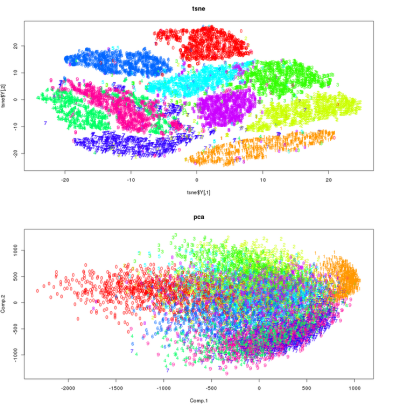
t-SNE is able to learn good, realistic manifolds as it is able to effectively capture the non-linear relationships and interactions in data, if they are present. t-SNE in its original form computes, specifically, a 2-dimensional projection / map. We can see a comparison of t-SNE and PCA in the below image. It is clear that PCA is inherently limited, since the projection into the principal subspace is linear. It is clear that t-SNE has much more effectively captured the structure of the data, and allowed for a much nicer, clearer visualization.
Some great resources for this topic can be found at: