Local Feature Encoding and Quantisation
In this post, I will describe local feature encoding and quantisation - why it is useful, where it is used, and some of the popular techniques used to perform it.
Feature quantisation is commonly used in domains such as image and video retrieval, however, it can be applied anywhere we would like to convert a variable number of local features into a single feature of uniform dimensionality.
Consider a set of images \(\{I_i\}^{n}_{i=1}\), and that we would like to obtain a fixed-length representation of each image so that we can index them quickly and easily by comparing these representation using some similarity measure. One common way to do this is to find interest points on the images, and compute the SIFT or SURF descriptors around those interest points. This means that each image will have a set of descriptors \(\{v_j\}_{j=1}^{n_i}\), where \(n_i\) is the number of descriptors found for image \(I_i\). It is clear that since the \(n_i\)s are not necessarily equal, we need some scheme to compute a fixed-length global representation of the image, using these local descriptors, in order, for example, to be able to compare similarity between images.
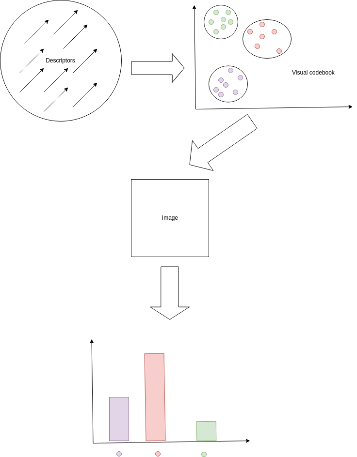
The most popular of these local feature encoding methods is bag-of-words (BoW). This is sometimes known as bag-of-visual-words, or bag-of-features. This technique is performed in the following manner. We sample a subset of the local descriptors across all images. Call this set \(S\). We then use the descriptors in \(S\) to estimate a K-Means clustering with \(K\) cluster centroids. These \(K\) centroids can be thought of as visual codebooks in the image feature space. Once we have learned this so-called visual codebook, we can then use it to compute a global, fixed-length representation of an image.
To compute the fixed-length representation, consider a particular image \(I_i\)’s descriptor set \(\{v_j\}_{j=1}^{n_i}\). We then compute a vector \(h \in \mathbb{R}^K\), where the \(i\)th dimension of \(h\) relates to the number of local descriptors of \(I_i\) that belong to \(i\)th visual word (i.e. cluster centroid) of the K-Means clustering. This is the quantisation part of the process. Determining what visual word a particular descriptor belongs to is achieved by computed distance between the descriptor and all the cluster centroids, using some distance metric (usually Euclidean distance) in the image feature space. This vector of counts is then L2-normalized to obtain the final, global, fixed-length representation of the image \(I_i\).
Other techniques exist to encode local features into global features such as Fisher vectors, and VLAD (vector of locally aggregated descriptors). Fisher vectors are the current state-of-the-art in this domain. However, they can quickly become very high-dimensional, as they are essentially a concatenation of partial derivatives of the parameters of a GMM (Gaussian mixture model) estimated with \(D\) modes in the image feature space. They are \(2 K D + K\)-dimensional, however, the \(K\) term is often discarded as these are the derivates of the GMM with respect to the mixture weights, and have been emprically shown to not provide much value to the representation. Thus, they are typically \(2 K D\)-dimensional. VLAD is a representation computed by quantising the residuals of the descriptors with respect to their assigned cluster centroids in a K-Means clustering of the data. They often result in similar performance to Fisher vectors, while being of a lower dimensionality and quicker to compute.
Some great resources for this topic can be found at: