SVMs: A Geometric Interpretation
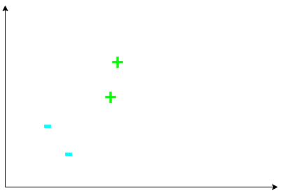
Consider a set of positive and negative samples from some dataset as shown above. How can we approach the problem of classifying these - and more importantly, unseen - samples as either positive or negative examples? The most intuitive way to do this is to draw a line / hyperplane between the between the positive and negative samples.
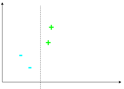
However, which line should we draw? We could draw this one:
or this one:
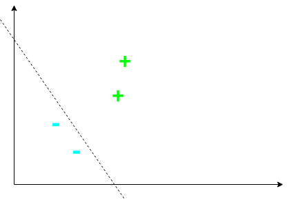
However, neither of the above seem like the best fit. Perhaps a line such that the boundary between the two classes is maximal is the optimal line?
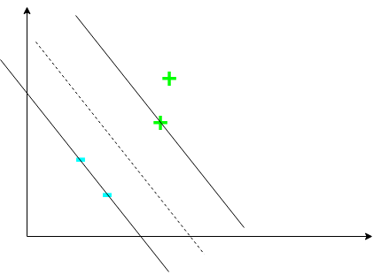
This line is such that the margin is maximized. This is the line an SVM attempts to find - an SVM attempts to find the maximum-margin separating hyperplane between the two classes. However, we need to construct a decision rule to classify examples. To do this, consider a vector \(\mathbf{w}\) perpendicular to the margin. Further, consider some unknown vector \(\mathbf{u}\) representing some example we want to classify:
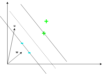
We want to know what side of the decision boundary \(\mathbf{u}\) is in order to classify it. To do this, we project it onto \(\mathbf{w}\) by computing \(\mathbf{w} \cdot \mathbf{u}\). This will give us a value that is proportional to the distance \(\mathbf{u}\) is, in the direction of \(\mathbf{w}\). We can then use this to determine which side of the boundary \(\mathbf{u}\) lies on using the following decision rule:
\[\mathbf{w} \cdot \mathbf{u} \ge c\]for some \(c \in \mathbb{R}\). \(c\) is basically telling us that if we are far enough away, we can classify \(\mathbf{u}\) as a positive example. We can rewrite the above decision rule as follows:
\[\mathbf{w} \cdot \mathbf{u} + b \ge 0\]where \(b = -c\).
But, what \(\mathbf{w}\) and \(b\) should we choose? We don’t have enough constraint in the problem to fix a particular \(\mathbf{w}\) or \(b\). Therefore, we introduce additional constraints:
\[\mathbf{w} \cdot \mathbf{x}_+ + b \ge 1\]and
\[\mathbf{w} \cdot \mathbf{x}_- + b \le -1\]These constraints basically force the function that defines our decision rule to produce a value of 1 or greater for positive examples, and -1 or less for negative examples.
Now, instead of dealing with two inequalities, we introduce a new variable, \(y_i\), for mathematical convenience. It is defined as:
\[y_i = \begin{cases} 1 & \text{positive example} \\ -1 & \text{negative example} \end{cases}\]This variable essentially encodes the targets of each example. We multiply both inequalities from above by \(y_i\). For the positive example constraint we get:
\[y_i (\mathbf{w} \cdot \mathbf{x}_i + b) \ge 1\]and for the negative example constraint we get:
\[y_i (\mathbf{w} \cdot \mathbf{x}_i + b) \ge 1\]which is the same constraint! The introduction of \(y_i\) has simplified the problem. We can rewrite this constraint as:
\[y_i (\mathbf{w} \cdot \mathbf{x}_i + b) - 1 \ge 0\]However, we go a step further by making the above inequality even more stringent:
\[y_i (\mathbf{w} \cdot \mathbf{x}_i + b) - 1 = 0\]The above equation constrains examples lying on the margins (known as support vectors) to be exactly 0. We do this because if a training point lies exactly on the margin, we don’t want to classify it as either positive or negative, since it’s exactly in the middle. We instead want such points to define our decision boundary. It is also clearly the equation of a hyperplane, which is what we want!
Keep in mind that our goal is to find the margin separating positive and negative examples to be as large as possible. This means that we will need to know the width of our margin so that we can maximize it. The following picture shows how we can calculate this width.
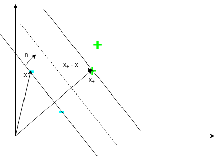
To calculate the width of the margin, we need a unit normal. Then we can just project \(\mathbf{x}_+ - \mathbf{x}_-\) onto this unit normal and this would exactly be the width of the margin. Luckily, vector \(\mathbf{w}\) was defined to be normal! Thus, we can compute the width as follows:
\[\text{width} = (\mathbf{x}_+ - \mathbf{x}_-) \cdot \frac{\mathbf{w}}{||\mathbf{w}||}\]where the norm ensures that \(\mathbf{w}\) becomes a unit normal. From earlier, we know \(y_i (\mathbf{w} \cdot \mathbf{x}_i + b) - 1 = 0\). Using this, simple algebra yields:
\[\mathbf{x}_+ \cdot \mathbf{w} = 1 - b\]and
\[- \mathbf{x}_- \cdot \mathbf{w} = 1 + b\]Thus, substituting into the expression for the width yields:
\[\text{width} = \frac{2}{||\mathbf{w}||}\]which is interesting! The width of our margin for such a problem depends only on \(\mathbf{w}\). Since we want to maximize the margin, we want:
\[\text{max} \frac{2}{||\mathbf{w}||}\]which is the same as
\[\text{max} \frac{1}{||\mathbf{w}||}\]which is the same as
\[\text{min} ||\mathbf{w}||\]which is the same as
\[\text{min} \frac{1}{2} ||\mathbf{w}||^2\]where we write it like this for mathematical convenience reasons that will become apparent shortly.
One easy approach to solve such an optimisation problem is using Lagrange multipliers. We first formulate our Lagrangian:
\[L(\mathbf{w}, b) = \frac{1}{2} ||\mathbf{w}||^2 - \sum_i \alpha_i [y_i (\mathbf{w} \cdot \mathbf{x}_i + b) - 1]\]We find the optimal settings for \(\mathbf{w}\) and \(b\) by computing the respective partial derivatives and setting them to zero. First, for \(\mathbf{w}\):
\[\frac{\partial L}{\partial \mathbf{w}} = \mathbf{w} - \sum_i \alpha_i y_i x_i = 0\]which implies that \(\mathbf{w} = \sum_i \alpha_i y_i x_i\). This means that \(\mathbf{w}\) is simply a linear combination of the samples! Now, for \(b\):
\[\frac{\partial L}{\partial b} = - \sum_i \alpha_i y_i = 0\]which implies that \(\sum_i \alpha_i y_i = 0\).
We could just stop here. We can solve the optimisation problem as is. However, we shall not do that! At least not yet. Let’s plug our expressions for \(\mathbf{w}\) and \(b\) back into the Lagrangian:
\[L = \frac{1}{2} (\sum_i \alpha_i y_i \mathbf{x}_i) \cdot (\sum_j \alpha_j y_j \mathbf{x}_j) - \sum_i \alpha_i y_i \mathbf{x}_i \cdot (\sum_j \alpha_j y_j \mathbf{x}_j) - \sum_i \alpha_i y_i b + \sum_i \alpha_i\]which, after some algebra, results in:
\[L = \sum_i \alpha_i - \frac{1}{2} \sum_i \sum_j \alpha_i \alpha_j y_i y_j \mathbf{x}_i \cdot \mathbf{x}_j\]What the above equation tells us is that the optimisation depends only on dot products of pairs of samples! This observation will prove key later on. Also, we should note that training examples that are not support vectors will have \(\alpha_i = 0\), as these examples do not effect or define the decision boundary.
Putting the expressions for \(\mathbf{w}\) and \(b\) back into our decision rule yields:
\[\sum_i \alpha_i y_i \mathbf{x}_i \cdot \mathbf{u} + b \ge 0\]which means the decision rule also depends only on dot products of pairs of samples! Another great benefit is that it is provable that this optimisation problem is convex - meaning we are guaranteed to always find global optima.
However, now a problem arises! The above optimisation problem assumes the data is linearly-separable in the input vector space. However, in most real-life scenarios, this assumption is simply untrue. We therefore have to adapt the SVM to accommodate for this, and to allow for non-linear decision boundaries. To do this, we introduce a transformation \(\phi\) which will transform the input vector into a (high-dimensional) vector space. It is in this vector space that we will attempt to find the maximum-margin line / hyperplane. In this case, we would simply need to swap the dot product \(\mathbf{x}_i \cdot \mathbf{x_j}\) in the optimisation problem with \(\phi(\mathbf{x}_i) \cdot \phi(\mathbf{x_j})\). We can do this solely because, as shown above, both the optimisation and decision rule depends only on dot products between pairs of samples. This is known as the kernel trick. Thus, if we have a function \(K\) such that:
\[K(\mathbf{x}_i, \mathbf{x}_j) = \phi(\mathbf{x}_i) \cdot \phi(\mathbf{x_j})\]then we don’t actually need to know the transformation \(\phi\) itself! We only need the function \(K\), which is known as a kernel function. This is why we can use kernels that transform the data into an infinite-dimensional space (such as the RBF kernel), because we are not computing the transformations directly. Instead, we simply use a special function (i.e. kernel function) to compute dot products in this space without needing to compute the transformations.
This kernel trick allows the SVM to learn non-linear decision boundaries, and the problem still clearly remains convex. However, even with the kernel trick, the SVM with such a formulation still assumes that the data in linearly-separable in this transformed space. Such SVMs are known as hard-margin SVMs. This assumption does not hold most the time for real-world data. Therefore, we arrive at the most common form of the SVM nowadays - the soft-margin SVMs. Essentially, so-called slack variables are introduced into the optimisation problem to control the amount of misclassification the SVM is allowed to make. For more information on soft-margin SVMs, see my blog post on the subject.
I highly recommend looking at this lecture if you would like to learn more about the concept behind SVMs.